
I’ve been demonstrating how you can build RAG pipelines with your existing relational data using our Oracle AI Database, without having to setup a completely separate Vector database, i.e. cough Pinecone, cough Postgres.
RAG pipelines allow you to augment your LLM’s context with your existing data from your own database – in our case, our Oracle AI Database.
Previously on thatJeffSmith…
- Build a ChatGPT Plugin for PowerPoint Search with Oracle AI
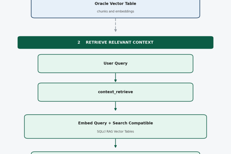
- Building a RAG pipeline on my Strava data for custom exercise training advice
Using Vectors/Maths to find related information is VERY powerful, but things can look similar, but still now be valid or as valid as other bits of information.
What IF instead of only relying on text chunks and their vectors via AI vector similarity search, we could ALSO use a knowledge graph (nodes and relationships) to model how information connects across documents, entities, or rows of our data?
Yes, Margaret, Oracle AI Database Supports Graph!
What you need to know:
- Standard SQL & Property Graphs: Oracle AI Database 26ai has full support for the SQL:2023 standard (
SQL/PGQand theGRAPH_TABLEoperator), allowing you to create property graphs from database views and query them using standard SQL syntax. - Graph information and support docs at Oracle.com
- Read the official Graph Blog
That ALSO means we can easily visualize how things are connected. This becomes super useful for doing things like, uncovering potential bank fraud.
Or if you’re a weirdo like me, you could spend a ton of time trying to see how I search my music collection based on descriptions and how related the music is by a couple of specific producers, like 2026 Rock’n’Roll HOF inductee Rick Rubin.
That’s what I want to show you today – a system that allows me to semantic search my vinyl music collection, but add a ranking ‘weight’ if said have music was also likely to have been influenced by Rick Rubin.
One SQL statement, three retrieval layers: relational facts, vector similarity and property-graph evidence, all inside a single, Oracle database.
1. The Data: My Record collection
I understand this is a personal post. If you’re reading this, imagine what relationships your data might hold, and how those could be unlocked.

If you need help on the imagination side, a couple of common use cases include:
- knowlege and document Q&A: LLM pulls info out of your powerpoints, word docs, etc, groups them into “communities”, and then you can ask questions that RAG alone would struggle with, because you can now see info that is linked across dozens or even thousands of docs, you can return more trusted answers
- customer support: graphs connect your products, versions, components, libraries, solutions, etc, and questions can be answered via similarity search. You know you’re more likely to get the right answer from the right document, because the graph has confirmed the relationship is direct or ‘very strong.’
But my use case is completely made up.
“I want something heavy and weird with political lyrics. What’ve you got?” And for giggles, if Rick Rubin or Matt Lunge touched it, or even came close to influencing it, that’s worth a signal bump in the results.
My query needs to perform 3 jobs, and those require 3 different patterns or shapes of data:
- Relational checks the facts (who, what year, which producer)
- Vectors find what matches a natural-language request
- Graph explains why a match is strong (evidence paths) – I don’t want just the facts, I want a text description of the match/relationship!
2. The data: a record collection as a relational model
I don’t have a lot of records, ~70 or so, but don’t feel bad for me, I spent WAY too much money acquiring those nostalgia-filled poster-shaped candy bars.
Simple rows and columns, just like you’re used to seeing and working with.
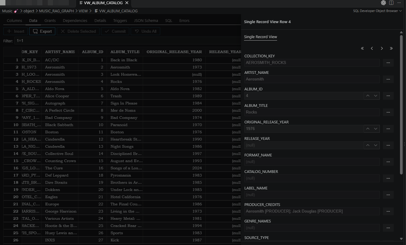
Code sample, the relational layer:
SELECT artist_name, album_title, original_release_year, producer_credits
FROM   vw_album_catalog
WHERE  producer_credits LIKE '%Rick Rubin%';
2. Chunking and Vectorizing the music
The artists and their albums have descriptions. I took these and vectorized them. Wait, what does that mean?
In this case it means I have a table with a VECTOR column that has vectors that describe text that was stored alongside it, that’s used to describe the music. My descriptions are on the shorter side, and weighted towards the genre, mood, beat, etc.
We calculated those Vectors in the database, as I have a sentence transformer available via SQL function, so an UPDATE TABLE is trivial to have our data available for AI Similarity Search.
Do the work:
UPDATE album_document
SET    embedding       = VECTOR_EMBEDDING(hr.all_minilm_l12_v2 USING content_text AS data),
       embedding_model = 'HR.ALL_MINILM_L12_V2 (all-MiniLM-L12-v2 ONNX, 384 FLOAT32)'
WHERE  embedding IS NULL;
Browsing the chunked data and their associated vectors:
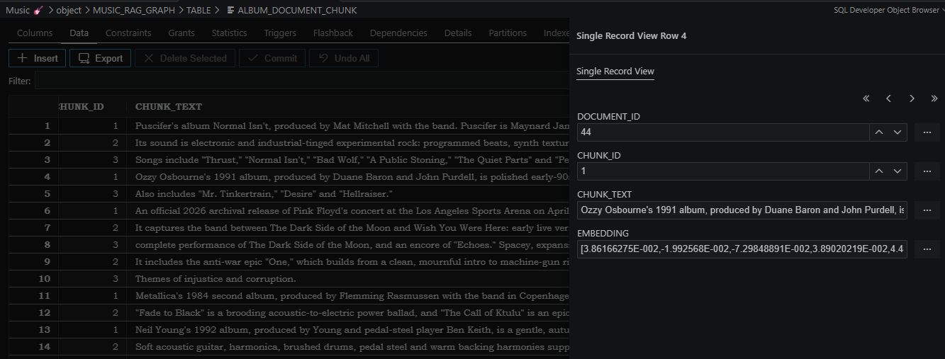
And querying this data, semantically, vs pattern matching, wild cards, or via RegEx functions would look like this –
SELECT d.album_id, ch.chunk_id,
       1 - VECTOR_DISTANCE(ch.embedding,
               VECTOR_EMBEDDING(hr.all_minilm_l12_v2
               USING 'quirky aggressive alternative metal with political lyrics' AS data),   -- >>>
COSINE) AS sim...Since my embedding model is available in the database (MiniLM-L12-v2 ONNX model (384 dimensions)), I can simply call the search string, the database will convert that to a VECTOR, and then use that to find other records that are similar.
3. First search, first lesson: one vector per document isn’t enough
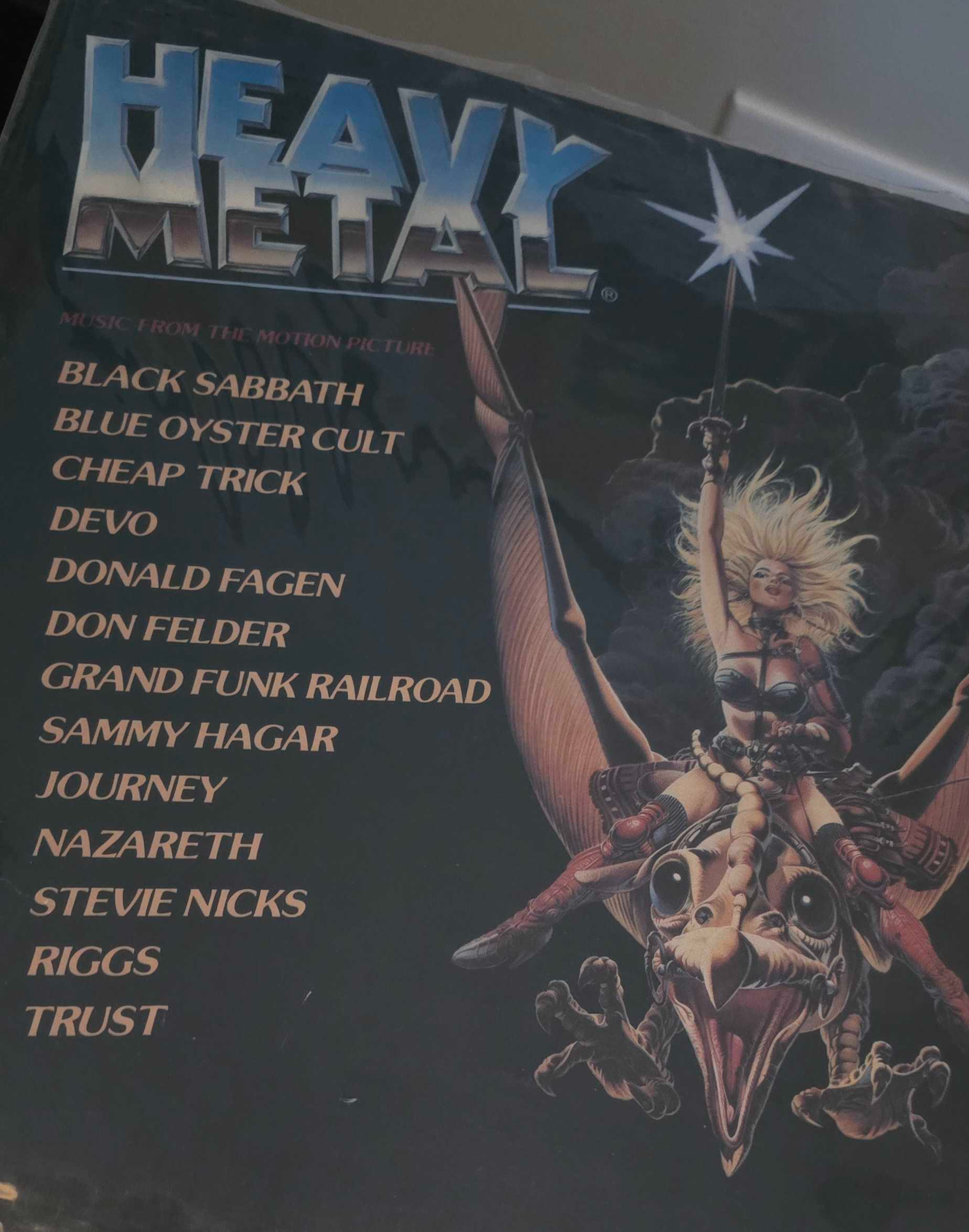
The LLMs are incredibly capable. Our first attempt at this failed, because I had an album that matched almost EVERY SINGLE search.
- My copy of the Heavy Metal movie soundtrack wins almost every search. Its description names a dozen genres, so its averaged vector sits close to everything.
- Smaller chunked descriptions, and keep only the most relevant chunks vs storing everything.
After applying a bit more selective set of descriptions, I started getting better search results.
| Query | Entire description #1 | Only the best Chunk #1 |
|---|---|---|
| heavy classical music | Heavy Metal OST (0.419) | Metallica, S&M (0.588) |
| funky danceable grooves | INXS, The Swing | Talking Heads, Stop Making Sense |
| dark depressing songs about addiction | Heavy Metal OST | Third Eye Blind (Mad Season now top 3) |
Code sample, chunking with DBMS_VECTOR_CHAIN:
INSERT INTO album_document_chunk (document_id, chunk_id, chunk_text)
SELECT d.document_id, jt.chunk_id, jt.chunk_data
FROM   album_document d,
       TABLE(dbms_vector_chain.utl_to_chunks(d.content_text,
             JSON('{"by":"words","max":"60","overlap":"0","split":"sentence","normalize":"all"}'))) c,
       JSON_TABLE(c.column_value, '$' COLUMNS (chunk_id NUMBER PATH '$.chunk_id',
                                               chunk_data VARCHAR2(4000) PATH '$.chunk_data')) jt;
Code sample, best-chunk vector search:
SELECT c.artist_name, c.album_title,
       ROUND(MAX(1 - VECTOR_DISTANCE(ch.embedding,
             VECTOR_EMBEDDING(hr.all_minilm_l12_v2 USING 'heavy classical music' AS data), COSINE)), 3) AS similarity
FROM   album_document_chunk ch
JOIN   album_document d   ON d.document_id = ch.document_id
JOIN   vw_album_catalog c ON c.album_id = d.album_id
GROUP  BY c.artist_name, c.album_title
ORDER  BY similarity DESC
FETCH FIRST 5 ROWS ONLY;
4. The graph: who worked with whom
We have in place the beginnings of my RAG pipeline. I’ve done this before, many times. Now it’s time to bulletproof this thing using the human relationships that tie these bands and their albums together.
To accomplish this, I’m going to need:
- A SQL property graph over the existing tables:
- artists,
- albums,
- tracks
- edges for “credited to”, “produced by”, “written by”, “contains track”
And the nice thing is I’m going to be able to do this WITHOUT having to copy any data around. That means not needing to maintain multiple systems, auth policies, ETL pipelines/replications, backup & recovery or patching mechanisms. All because we have the data in a single database, accessible via a single SQL interface.
One of my property graphs looks like this:
CREATE OR REPLACE PROPERTY GRAPH vinyl_graph
  VERTEX TABLES (
    music_artist KEY (artist_id) LABEL artist
      PROPERTIES (artist_id, display_name, artist_type, origin_country),
    album KEY (album_id) LABEL album
      PROPERTIES (album_id, title, original_release_year),
    track KEY (track_id) LABEL track
      PROPERTIES (track_id, disc_number, track_number, track_title, duration_seconds)
  )
  EDGE TABLES (
    album_credit KEY (album_id, artist_id, credit_role)
      SOURCE KEY (album_id) REFERENCES album (album_id)
      DESTINATION KEY (artist_id) REFERENCES music_artist (artist_id)
      LABEL credited_to,
    album_producer KEY (album_id, producer_id, producer_role)
      SOURCE KEY (album_id) REFERENCES album (album_id)
      DESTINATION KEY (producer_id) REFERENCES music_artist (artist_id)
      LABEL produced_by,
    track AS album_track KEY (track_id)
      SOURCE KEY (album_id) REFERENCES album (album_id)
      DESTINATION KEY (track_id) REFERENCES track (track_id)
      LABEL contains_track,
    track_songwriter KEY (track_id, songwriter_id, credit_role)
      SOURCE KEY (track_id) REFERENCES track (track_id)
      DESTINATION KEY (songwriter_id) REFERENCES music_artist (artist_id)
      LABEL written_by,
    artist_relationship KEY (relationship_id)
      SOURCE KEY (source_artist_id) REFERENCES music_artist (artist_id)
      DESTINATION KEY (target_artist_id) REFERENCES music_artist (artist_id)
      LABEL related_to
      PROPERTIES (relationship_type, evidence_note, source_url)
  );
Not shown: record label, genre and Hall of Fame vertices.
And now to query this info, let’s do a simple GRAPH_TABLE search.
This query answers a question: “Which records in my collection are connected to Rick Rubin, even though he didn’t produce them?” Think the 6 degrees of Kevin Bacon game, but for Rick.
The SQL allows us to follow a trail:
- Start with Rick Rubin.
- Find a band he has worked with. Example: Rubin produced AC/DC’s album Ballbreaker (I have the CD for this, but not the LP).
- Find an album by that band in my collection. I own AC/DC’s Back in Black.
- See who produced that album. Back in Black was produced by Mutt Lange.
- Find another album that producer made. Mutt Lange also produced Def Leppard’s Pyromania.
SELECT DISTINCT anchor, band, via_album, shared_producer, related_album
FROM GRAPH_TABLE (vinyl_graph
  MATCH (r IS artist) -[rel IS related_to]-> (band IS artist)
        <-[IS credited_to]- (a1 IS album) -[IS produced_by]-> (prod IS artist)
        <-[IS produced_by]- (a2 IS album)
  WHERE r.display_name = 'Rick Rubin'
    AND a1.album_id <> a2.album_id AND prod.artist_id <> band.artist_id
  COLUMNS (r.display_name AS anchor, band.display_name AS band, a1.title AS via_album,
           prod.display_name AS shared_producer, a2.title AS related_album));
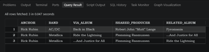
When I run this, only the first row is really interesting, because duh, ‘Metallica is related to Metallica.’ If I were tracking my CD collection, there’d be way more connections, but I don’t have the time or energy to diary that!
5. Sorry, it’s math time, but only a very little bit
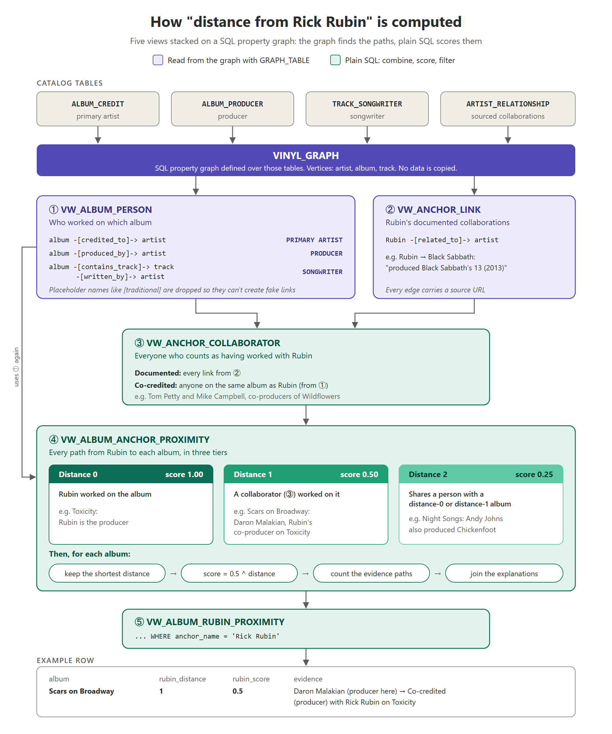
We need to measure just how far away really is Rick Rubin. And so I need to define some [arbitrary] rules:
- 0: Rubin worked on it (producer, artist or songwriter)
- 1: someone who worked with Rubin worked on it, either a documented collaboration or a co-credit on the same record
- 2: one more person removed
Example: Rick Rubin co-produced Toxicity with Daron Malakian. Malakian produced Scars on Broadway, so that record is distance 1.
Scores halve per hop (1.0, 0.5, 0.25).
Every score brings alongside it a trail.
The co-credit path :
SELECT anchor, anchor_album, collaborator, other_album
FROM GRAPH_TABLE (vinyl_graph
  MATCH (r IS artist) <-[IS produced_by|credited_to]- (a1 IS album)
        -[IS produced_by|credited_to]-> (p IS artist)
        <-[IS produced_by|credited_to]- (a2 IS album)
  WHERE r.display_name = 'Rick Rubin'
    AND p.artist_id <> r.artist_id AND a2.album_id <> a1.album_id
  COLUMNS (r.display_name AS anchor, a1.title AS anchor_album,
           p.display_name AS collaborator, a2.title AS other_album));
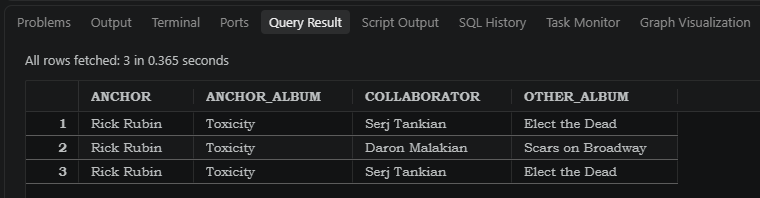
Our results: Toxicity → Daron Malakian → Scars on Broadway; Toxicity → Serj Tankian → Elect the Dead.
Code sample, querying the evidence view:
SELECT c.album_title, p.rubin_distance, p.evidence
FROM   vw_album_rubin_proximity p
JOIN   vw_album_catalog c ON c.album_id = p.album_id
ORDER  BY p.rubin_distance, c.album_title;
This query is deceptively simply. It’s querying a view that ties into FOUR more views, It’s in those views that the ‘distance’ is computed.
It’s at this point you need to remember I am not a “Graph Guy.” There may very well be a better way to handle this. I’m just giving my collaborator, Codex/GPT-6 Luna, a VERY large amount of leeway on how to achieve my goals.
6. Seeing the graph in SQL Developer
Let’s look at another example.
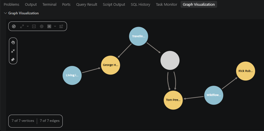
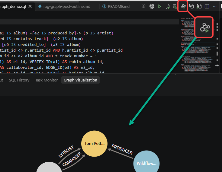
Rick Rubin → produced Wildflowers → Tom Petty also made → “Handle With Care” → Traveling Wilburys Vol. 1 → with George Harrison → who also did Living in the Material World.
Query
SELECT *
FROM GRAPH_TABLE (vinyl_graph
  MATCH (r IS artist) <-[e1 IS produced_by]- (a1 IS album) -[e2 IS produced_by]-> (p IS artist)
        <-[e3 IS written_by]- (t IS track) <-[e4 IS contains_track]- (a2 IS album)
        -[e5 IS produced_by]-> (h IS artist) <-[e6 IS credited_to]- (a3 IS album)
  WHERE r.display_name = 'Rick Rubin' AND p.artist_id <> r.artist_id AND h.artist_id <> p.artist_id
    AND a2.album_id <> a1.album_id AND a3.album_id <> a2.album_id AND t.track_number = 1
  COLUMNS (VERTEX_ID(r) AS rubin_id, EDGE_ID(e1) AS e1_id, VERTEX_ID(a1) AS rubin_album_id,
           EDGE_ID(e2) AS e2_id, VERTEX_ID(p) AS collaborator_id, EDGE_ID(e3) AS e3_id,
           VERTEX_ID(t) AS track_id, EDGE_ID(e4) AS e4_id, VERTEX_ID(a2) AS bridge_album_id,
           EDGE_ID(e5) AS e5_id, VERTEX_ID(h) AS bridge_person_id, EDGE_ID(e6) AS e6_id,
           VERTEX_ID(a3) AS far_album_id));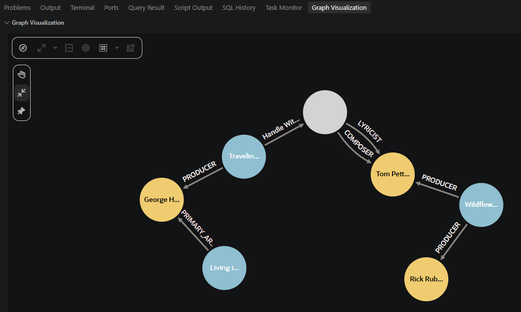
Or we can connect Cinderella to the Red Hot Chilipeppers… via Rubin and RHCP’s drummer, Chad Smith.
Query:
SELECT *
FROM GRAPH_TABLE (vinyl_graph
  MATCH (r IS artist) <-[e1 IS produced_by]- (a1 IS album) -[e2 IS contains_track]-> (t1 IS track)
        -[e3 IS written_by]-> (p IS artist) <-[e4 IS written_by]- (t2 IS track) <-[e5 IS contains_track]- (a2 IS album)
        -[e6 IS produced_by]-> (h IS artist) <-[e7 IS produced_by]- (a3 IS album)
  WHERE r.display_name = 'Rick Rubin' AND p.display_name = 'Chad Smith' AND h.display_name = 'Andy Johns'
    AND a2.album_id <> a1.album_id AND a3.album_id <> a2.album_id AND t1.track_title = 'Give It Away'
  COLUMNS (VERTEX_ID(r) AS rubin_id, EDGE_ID(e1) AS e1_id, VERTEX_ID(a1) AS rubin_album_id,
           EDGE_ID(e2) AS e2_id, VERTEX_ID(t1) AS rubin_track_id, EDGE_ID(e3) AS e3_id,
           VERTEX_ID(p) AS collaborator_id, EDGE_ID(e4) AS e4_id, VERTEX_ID(t2) AS bridge_track_id,
           EDGE_ID(e5) AS e5_id, VERTEX_ID(a2) AS bridge_album_id, EDGE_ID(e6) AS e6_id,
           VERTEX_ID(h) AS bridge_producer_id, EDGE_ID(e7) AS e7_id, VERTEX_ID(a3) AS far_album_id));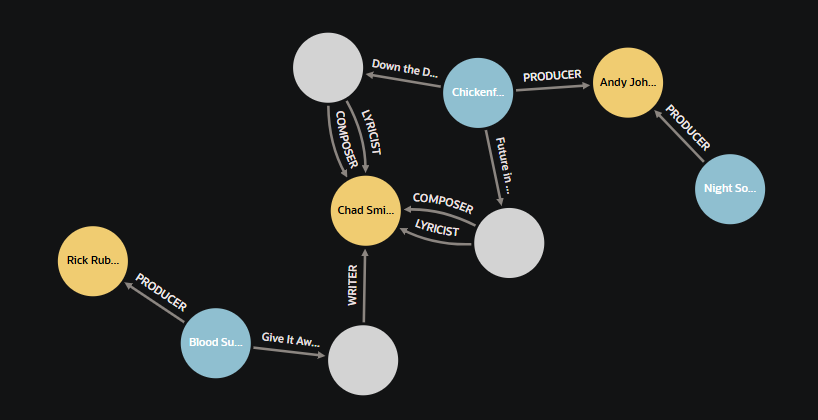
💡Tip: if you install the SQL Developer Graph Extension, then you get a new Execute button on the SQL Worksheet, and the Visualization display alongside your query results.
7. Putting it together: one SQL statement, three layers
Ok so that was a lot to slog through, but the first two parts were hopefully familiar for you. And if the Graph stuff is giving you a headache because you’re brand new to it (like me), ask your Agent to help!
So I have a big query, that looks for my records based on a description, and it takes in a request and gives ranked answers out, with descriptions of the match via vector and the trust level via graph.
WITH vector_hits AS (
  SELECT /*+ NO_MERGE */ d.album_id, ch.chunk_id,
         1 - VECTOR_DISTANCE(ch.embedding,
               VECTOR_EMBEDDING(hr.all_minilm_l12_v2
                 USING 'quirky aggressive alternative metal with political lyrics' AS data),
               COSINE) AS sim
  FROM   album_document_chunk ch
  JOIN   album_document d ON d.document_id = ch.document_id
),
candidates AS (
  SELECT album_id,
         MAX(sim) AS vector_sim,
         MAX(chunk_id) KEEP (DENSE_RANK FIRST ORDER BY sim DESC) AS best_chunk_id
  FROM   vector_hits
  GROUP  BY album_id
  ORDER  BY vector_sim DESC
  FETCH FIRST 10 ROWS ONLY
)
SELECT RANK() OVER (ORDER BY c.vector_sim + b.producer_boost DESC) AS final_rank,
       RANK() OVER (ORDER BY c.vector_sim DESC)                    AS vector_rank,
       cat.artist_name, cat.album_title,
       ROUND(c.vector_sim, 3)                    AS vector_sim,
       b.rubin_distance,
       ROUND(c.vector_sim + b.producer_boost, 3) AS final_score,
       rp.evidence                               AS rubin_evidence,
       ch.chunk_text                             AS why_it_matched
FROM   candidates c
JOIN   vw_album_catalog        cat ON cat.album_id = c.album_id
JOIN   vw_album_producer_boost b   ON b.album_id   = c.album_id
LEFT JOIN vw_album_rubin_proximity rp ON rp.album_id = c.album_id
JOIN   album_document d        ON d.album_id = c.album_id AND d.document_kind = 'DESCRIPTION'
JOIN   album_document_chunk ch ON ch.document_id = d.document_id AND ch.chunk_id = c.best_chunk_id
ORDER  BY final_rank;
Let’s look at the results now.
| Final | Vector rank | Album | Rubin distance | Note |
|---|---|---|---|---|
| 1 | 1 | Scars on Broadway | 1 | Malakian co-produced Toxicity |
| 2 | 2 | Toxicity | 0 | Rubin produced |
| 3 | 3 | Paranoid | 1 | Rubin produced Sabbath’s 13 |
| 4 | 5 | Elect the Dead | 1 | moved up past Autograph |
| 5 | 10 | Danzig 4 | 0 | 10th → 5th |
| 6 | 4 | Sign In Please (Autograph) | — | no pedigree, drops |
- Vector finds the System of a Down “family.”
- The graph lifts Elect the Dead past Autograph, and Danzig 4 from 10th to 5th.
- Autograph is a good text match but has no pedigree, so it drops.
Note that the distance metric only influences the ranking. I use a computed PRODUCER_SCORE value that takes the distance and multiplies that by 0.08 – and that is used to influence the ranking. We started with a 0.15, but that ended up being way too strong, as any graph relationship would automatically win out regardless of how good the vector similarity was.
Example, looking for a ‘harmonica’ song, would always bring back System of a Down’s Toxicity album, because Rick Rubin’s influence for the vector ‘matched’ results. And I can tell you there’s pretty much Zero harmonica involved there.
Another thing to keep in mind, if the Vector ‘misses’ a good answer, no strength in the graph side will allow that record to surface to the Agent. The similarity search is the first and overriding filter.
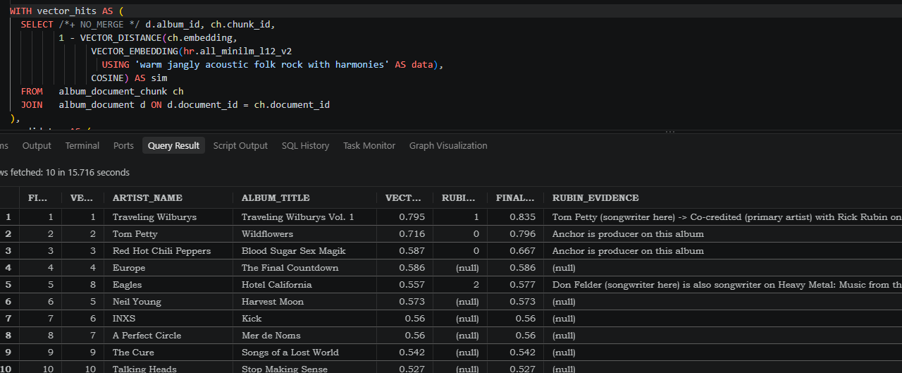
Another test run –
Second example: “warm jangly acoustic folk rock with harmonies” → Traveling Wilburys Vol. 1 #1 (distance 1 through Petty), Wildflowers #2.
Summary and parting thoughts
I allowed my creativity to perhaps go too far here, but really you’re only ever limited by your ideas these days, right? So think about the relationships your data, documents, media have, and how those could be used to verify or influence the information a Vector similarity search might return.
It seems a good bit of our jobs today is context engineering. How can we get the BEST information to our LLM, so we can expect the best, and trusted outcomes?
One of the things I found super useful as I worked through this, was the ‘show me the evidence’ component. The database doesn’t just have to use the relationships defined in the GRAPH table functions, it can ALSO return those relationships back in the query results itself – which can then be shared back to your Agent as context.
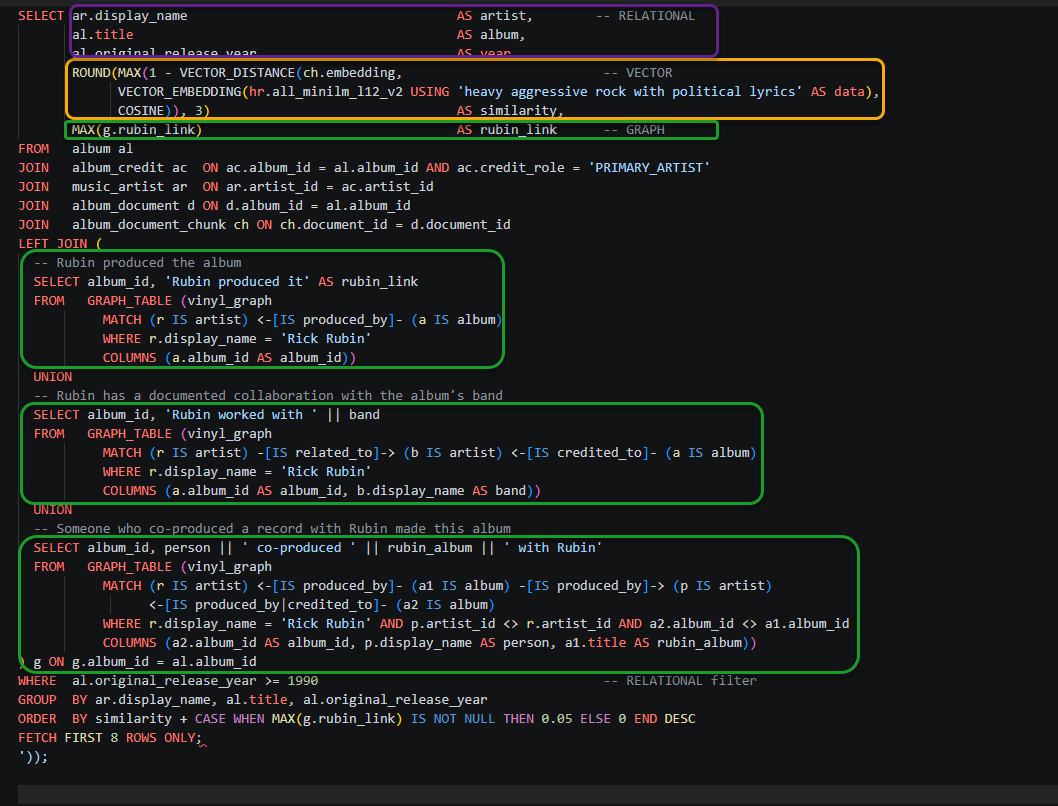
Finally, I wanted to end by sharing what a simplified version of what I was doing looks like, without relying on the VIEWS we created, which obscured a good bit of the GRAPH bits.
And finally, finally, I wanted to share with you some other Graph resources you may find useful: